3. Case study: colocalization analysis in prostate cancer

Before we start.

All we need to prepare include three parts:

GWAS summary statistics dataset.
Tissue of interest.
Following three installed packages.

library(xQTLbiolinks)
library(coloc)
library(hyprcoloc)
library(data.table)
library(stringr)
library(R.utils)
library(TxDb.Hsapiens.UCSC.hg38.knownGene)
library(VariantAnnotation)

Prostate cancer is one of the most common cancers in men. Prostate cancer pathogenesis involves both heritable and environmental factors. The molecular events involved in the development or progression of prostate cancer are still unclear. In this example, we aim to figure out the causal variants and genes assocaited with prostate cancer, and to uncover potential molecular mechanisms of regulation.

For data preparation, we download summary statistics dataset of a GWAS study (GCST006085) of prostate cancer from GWAS category and load the dataset in R with data.table package. Correspondingly, we chose tissue Prostate for study. We retain the variants with dbSNP id (start with rs), and a data.table object named gwasDF of 13,498,990 (rows) x 7 (cols) is loaded.

gwasDF <- fread("29892016-GCST006085-EFO_0001663-build37.f.tsv.gz")
# extract columns.
gwasDF<- gwasDF[str_detect(variant_id, "^rs"),.(rsid=variant_id, chrom=chromosome, position= base_pair_location, pValue=p_value, AF=effect_allele_frequency, beta, se= standard_error)]
# tissue:
tissueSiteDetail="Prostate"

head(gwasDF)

#>           rsid chrom position  pValue     AF    beta     se
#> 1: rs145072688     1    10352 0.46280 0.5753 -0.0094 0.0128
#> 2: rs376342519     1    10616 0.41070 0.0066  0.0572 0.0696
#> 3: rs201725126     1    13116 0.84470 0.8255 -0.0035 0.0178
#> 4: rs200579949     1    13118 0.84470 0.8255 -0.0035 0.0178
#> 5:  rs75454623     1    14930 0.61880 0.4772 -0.0065 0.0131
#> 6: rs199856693     1    14933 0.02721 0.0407 -0.0794 0.0360

Now we can perform quality control for this GWAS dataset by estimating the genomic inflation factor, validating QQ-plot and PZ-plot using xQTLbiolinks.

xQTLvisual_qqPlot(gwasDF[,.(pValue)])
xQTLvisual_PZPlot(gwasDF[,.(pValue, beta, se)])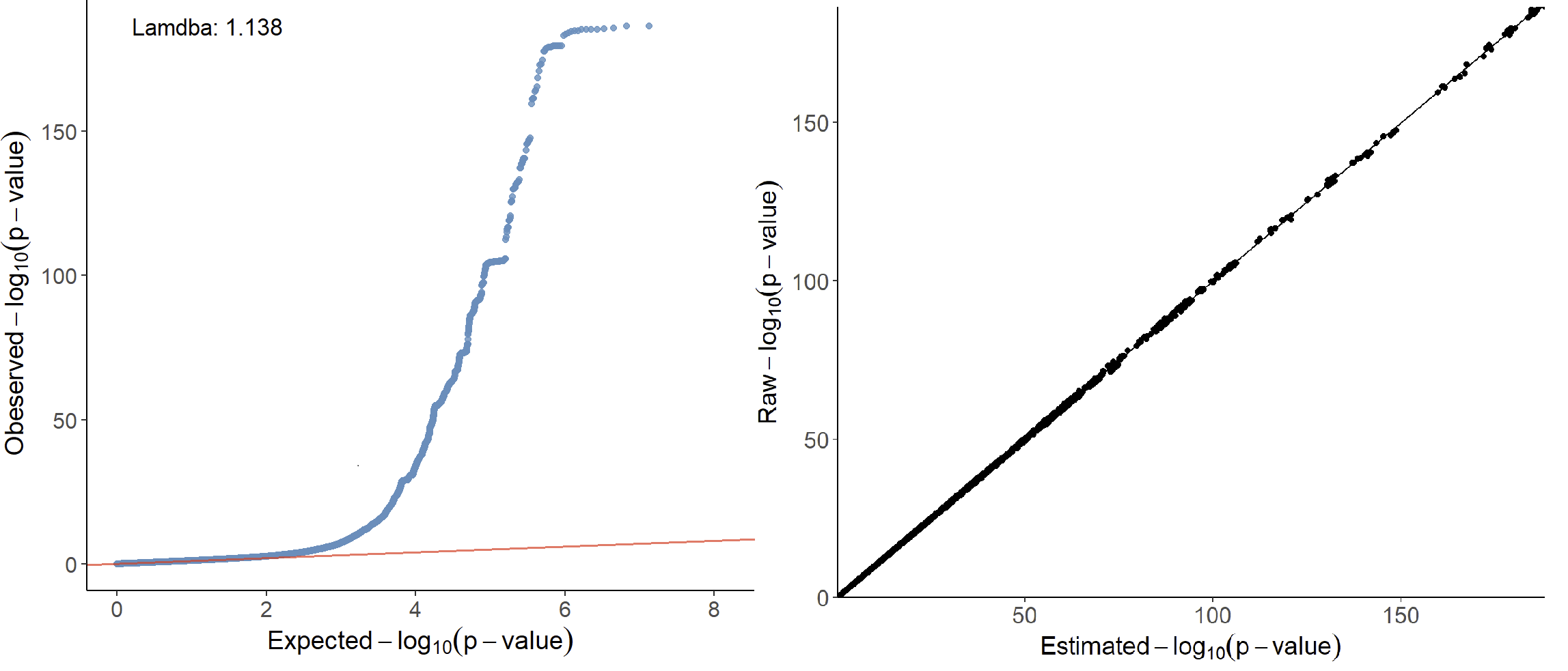

Left is the QQ-plot. The x-axis of the QQ-plot represents the expected p-values under the null hypothesis, while the y-axis represents the observed p-values from the GWAS summary statistics data. There is a significant deviation from the diagonal line, which indicates potential variations from the null hypothesis that may result from true associations or LD. The genomic inflation factor (lambda) is labeled in the top left of the QQ-plot, and a lambda value of 1.138 indicating no strong population stratification. Right is the PZ plot, the observed p-values on the y-axis and the corresponding p-values derived from z-scores that estimated by beta and se on the x-axis. A strong concordance can be observed between the observed p-values and those calculated from Z-scores.

Genomic annotation of the significant signals can be conducted using xQTLanno_genomic:

Step 1: Identify sentinel SNPs:

Sentinel SNP is the most prominent signal within a given genome range, and is usually in high LD with causal variants. By default, xQTLbiolinks detect sentinel snps that with the p-value < 5e-8 and SNP-to-SNP distance > 10e6 bp. Note: For in this example, due to the inconsistent genome version between the GWAS dataset (GRCh37) and eQTL associations (GRCh38) from eQTL category, conversion of genome version is required, and can be conducted using xQTLanalyze_getSentinelSnp with genomeVersion="grch37" and grch37To38=TRUE (package rtracklayeris required):

sentinelSnpDF <- xQTLanalyze_getSentinelSnp(gwasDF, centerRange=1e6,
                                            genomeVersion="grch37", grch37To38=TRUE)

A total of 94 sentinel SNPs are detected.

head(sentinelSnpDF)

#>           rsid  chr  position    pValue    maf    beta     se
#> 1:  rs55664108 chr1 204587862 8.572e-25 0.7157  0.0912 0.0089
#> 2:  rs35296356 chr1 150601662 3.355e-14 0.3384 -0.0690 0.0091
#> 3:  rs34579442 chr1 153927424 4.478e-14 0.6637 -0.0655 0.0087
#> 4: rs146564277 chr1 155051619 1.577e-12 0.0301 -0.1850 0.0262
#> 5:  rs34848415 chr1 205762038 2.893e-09 0.5231 -0.0501 0.0084
#> 6:  rs56391074 chr1  87745032 1.659e-08 0.6298 -0.0466 0.0082

Step 2: Identify trait genes for each sentinel SNPs:

Trait genes are genes that located in the range of 1Mb (default, can be changed with parameter detectRange) of sentinel SNPs. In order to reduce the number of trait genes and thus reduce the running time, we take the overlap of eGenes and trait genes as the final output of the function xQTLanalyze_getTraits:

traitsAll <- xQTLanalyze_getTraits(sentinelSnpDF, detectRange=1e6, tissueSiteDetail=tissueSiteDetail)

Totally, 898 associations between 835 traits genes and 92 sentinel SNPs are detected

head(traitsAll)

#>          rsid  chr  position    pValue    maf    beta     se       gencodeId
#> 1: rs34848415 chr1 205762038 2.893e-09 0.5231 -0.0501 0.0084 ENSG00000261000
#> 2: rs34848415 chr1 205762038 2.893e-09 0.5231 -0.0501 0.0084 ENSG00000263528
#> 3: rs34848415 chr1 205762038 2.893e-09 0.5231 -0.0501 0.0084 ENSG00000162877
#> 4: rs34848415 chr1 205762038 2.893e-09 0.5231 -0.0501 0.0084 ENSG00000117280
#> 5: rs34848415 chr1 205762038 2.893e-09 0.5231 -0.0501 0.0084 ENSG00000069275
#> 6: rs55664108 chr1 204587862 8.572e-25 0.7157  0.0912 0.0089 ENSG00000281406

Step 3: Conduct colocalization analysis with eQTL:

Following three steps of colocalization analysis are encapsulated in one function xQTLanalyze_coloc:

Retrieved all associations from EBI eQTL catalogue for a specified gene.
Merge the data.frame of GWAS and eQTL by rsid.
Perform colocalization analysis using coloc and hyprcoloc methods.

For above 835 trait genes, a for loop can be used to get these genes’ outputs of colocalization analysis (this may take several minutes):

# All genes:
genesAll<- xQTLquery_gene(unique(traitsAll$gencodeId))
setindex(gwasDF, rsid) # speed up merging
# A data.table to save results:
colocResultAll <- data.table()
for(i in 1:nrow(genesAll)){
  # eQTL of the gene i
  eQTL_i <- xQTLdownload_eqtlAllAsso(genesAll[i]$gencodeId, geneType = "gencodeId", tissueLabel=tissueSiteDetail, withB37VariantId = FALSE, data_source="liLab")
  gwasDF_i <- gwasDF[rsid  %in% eQTL_i$rsid,]
  if(is.null(eQTL_i)){next()}; if(nrow(gwasDF_i)==0){next()}
  eQTL_i <- merge(eQTL_i, gwasDF_i[,.(rsid, chrom, position)], by ="rsid")[,.(rsid, chrom, position, pValue, maf, beta, se)]
  # using both method coloc and hyprcoloc to perform colocalization analysis
  colocResult_i <- xQTLanalyze_coloc_diy(gwasDF = gwasDF_i, qtlDF = eQTL_i, method="Both")
  # 
  if(!is.null(colocResult_i)){ 
      colocResult_i <- colocResult_i$coloc_Out_summary
      colocResult_i <- cbind(genesAll[i,c("geneSymbol","gencodeId")], colocResult_i)
      colocResultAll <- rbind(colocResultAll, colocResult_i)}
  message(" == Id: ",i,"/",nrow(genesAll)," == Gene:",genesAll[i]$gencodeId)
}

In this case, we invoke two methods to conduct colocalization analysis, (1). coloc that estimates the posterior support of variants for each hypothesis: H0,H1,H2,H3,H4:

H0 : neither trait has a genetic association in the region
H1: only trait 1 has a genetic association in the region
H2: only trait 2 has a genetic association in the region
H3: both traits are associated, but with different causal variants
H4: both traits are associated and share a single causal variant

and (2). hyprcoloc that calculates the posterior probability that all traits share a causal variant.

Output is a data.table object that combined all results of colocOut of all genes.

head(colocResultAll)

#>       geneSymbol          gencodeId nsnps    PP.H0.abf    PP.H1.abf
#> 1: RP11-534L20.5  ENSG00000261000.1  4472 2.179842e-12 4.815048e-09
#> 2:         IKBKE  ENSG00000263528.7  4505 5.794749e-05 1.280001e-01
#> 3:        PM20D1 ENSG00000162877.12  5007 3.101352e-13 6.851499e-10
#> 4:         RAB29 ENSG00000117280.12  4998 2.696451e-11 5.957032e-08
#> 5:        NUCKS1 ENSG00000069275.12  5002 2.005928e-07 4.431533e-04
#> 6:       BLACAT1  ENSG00000281406.1  5011 4.875521e-19 4.875783e-01
#>       PP.H2.abf  PP.H3.abf    PP.H4.abf candidate_snp  SNP.PP.H4 hypr_posterior
#> 1: 4.522413e-04 0.99895403 0.0005937237     rs6693843 0.19259384         0.0001
#> 2: 3.939882e-04 0.87027865 0.0012693057      rs823121 0.07040552         0.0000
#> 3: 8.561368e-05 0.18832593 0.8115884566     rs1772159 0.39272007         0.5931
#> 4: 1.329558e-05 0.02840117 0.9715854781      rs708723 0.36167886         0.9428
#> 5: 1.253436e-05 0.02671831 0.9728258014      rs823154 0.42379078         0.9364
#> 6: 4.805752e-19 0.48056911 0.0318526046      rs930947 0.12798834         0.0039
#>    hypr_regional_prob hypr_candidate_snp hypr_posterior_explainedBySnp
#> 1:             0.2374          rs6693843                        0.2379
#> 2:             0.0057           rs823121                        0.0661
#> 3:             0.9995          rs1772159                        0.3313
#> 4:             1.0000           rs708723                        0.4030
#> 5:             0.9993           rs823154                        0.4423
#> 6:             0.0353          rs4245739                        0.1158

We can see that the two methodologies’ outcomes are quite consistent. With a threshold of 0.75 for coloc and 0.5 for hyprcoloc, a total of 26 colocalized genes are shared.

To save time and go through this case as soon as possible, you can get the above result directly with:

colocResultAll <- fread("http://bioinfo.szbl.ac.cn/xQTL_biolinks/xqtl_data/colocResultAll.txt")

Step 4: Visualization of the results:

We considered colocalization tests with a posterior probability of hypothesis 4 (PPH4.ABF) > 0.75 & hypr_posterior > 0.5 as having strong or moderate evidence for colocalization.

colocResultsig <- colocResultAll[PP.H4.abf>0.75 & hypr_posterior>0.5][order(-PP.H4.abf)]

There are 26 trait genes that are associated and share a single causal variant:

head(colocResultsig)

#>       geneSymbol          gencodeId nsnps    PP.H0.abf    PP.H1.abf
#> 1:          MMP7  ENSG00000137673.8  7108 4.037711e-17 8.285257e-05
#> 2: CTC-435M10.12  ENSG00000277744.1  4676 2.078933e-20 2.421163e-03
#> 3:      PPP1R14A ENSG00000167641.10  5034 5.328594e-34 2.988721e-07
#> 4:        GEMIN4 ENSG00000179409.10  6169 9.325967e-19 1.409617e-03
#> 5:          GGCX ENSG00000115486.11  5389 9.622300e-27 3.521949e-09
#> 6:          TBX1 ENSG00000184058.12  6044 1.851045e-09 1.456683e-07
#>       PP.H2.abf    PP.H3.abf PP.H4.abf candidate_snp SNP.PP.H4 hypr_posterior
#> 1: 6.360696e-16 0.0003055833 0.9996116    rs11568818 1.0000000         0.9993
#> 2: 1.588664e-20 0.0008534614 0.9967254     rs2079811 0.9999764         0.9923
#> 3: 8.166955e-30 0.0035842959 0.9964154     rs4802297 0.2683674         0.9911
#> 4: 2.672611e-18 0.0030440968 0.9955463     rs2740358 0.9493232         0.9869
#> 5: 2.411952e-20 0.0078360511 0.9921639    rs10175792 0.3177452         0.9830
#> 6: 2.233151e-04 0.0165906223 0.9831859     rs2238775 0.2005480         0.9778
#>    hypr_regional_prob hypr_candidate_snp hypr_posterior_explainedBySnp
#> 1:             0.9998         rs11568818                        1.0000
#> 2:             0.9943          rs2079811                        1.0000
#> 3:             1.0000          rs4802297                        0.2738
#> 4:             0.9960          rs2740358                        0.8927
#> 5:             1.0000         rs10175792                        0.3449
#> 6:             0.9995          rs2238775                        0.3230

All these genes’ details can be fetched with xQTLquery_gene:

outGenes <- xQTLquery_gene(colocResultsig$gencodeId)

Add the value of PPH4 for each gene, and remove non-protein-coding genes:

outGenes <- merge(colocResultsig[,c("gencodeId", "PP.H4.abf", "candidate_snp", "SNP.PP.H4", "hypr_posterior")], 
                  outGenes[,c("geneSymbol", "gencodeId", "entrezGeneId", "geneType")], by="gencodeId", sort=FALSE)
outGenes <- outGenes[geneType =="protein coding"]

outGenes

#>              gencodeId PP.H4.abf candidate_snp  SNP.PP.H4 hypr_posterior
#>  1:  ENSG00000137673.8 0.9996116    rs11568818 0.99999996         0.9993
#>  2: ENSG00000167641.10 0.9964154     rs4802297 0.26836743         0.9911
#>  3: ENSG00000179409.10 0.9955463     rs2740358 0.94932317         0.9869
#>  4: ENSG00000115486.11 0.9921639    rs10175792 0.31774517         0.9830
#>  5: ENSG00000184058.12 0.9831859     rs2238775 0.20054800         0.9778
#>  6: ENSG00000069275.12 0.9728258      rs823154 0.42379078         0.9364
#>  7: ENSG00000117280.12 0.9715855      rs708723 0.36167886         0.9428
#>  8: ENSG00000099331.13 0.9713063    rs11666569 0.25871794         0.9293
#>  9: ENSG00000184012.11 0.9660070     rs6517673 0.38159830         0.9127
#> 10:  ENSG00000172613.7 0.9576434    rs35826789 0.92558434         0.9038
#> 11: ENSG00000155749.12 0.9561720     rs7560328 0.22497345         0.8966
#> 12: ENSG00000204536.13 0.9366182     rs2517985 0.13110756         0.7333
#> 13:  ENSG00000180535.3 0.9361589     rs6465657 0.17430973         0.8643
#> 14: ENSG00000003400.14 0.9105858    rs12620010 0.37295865         0.7922
#> 15: ENSG00000101751.10 0.9084474     rs3730783 0.09578602         0.8321
#> 16: ENSG00000152601.17 0.8906783    rs73011743 0.03316094         0.7482
#> 17: ENSG00000136819.15 0.8812364    rs13300897 0.15189809         0.7313
#> 18: ENSG00000115648.13 0.8654407    rs72620824 0.54349674         0.7378
#> 19: ENSG00000198625.12 0.8209748     rs2169137 0.14030719         0.6086
#> 20: ENSG00000162877.12 0.8115885     rs1772159 0.39272007         0.5931
#> 21: ENSG00000065060.16 0.7949202   rs112283401 0.03978575         0.6114
#> 22: ENSG00000080546.13 0.7811190     rs6935782 0.08037725         0.6257
#> 23: ENSG00000118961.14 0.7700294     rs9306895 0.54356363         0.7300
#>              gencodeId PP.H4.abf candidate_snp  SNP.PP.H4 hypr_posterior
#>     geneSymbol entrezGeneId       geneType
#>  1:       MMP7         4316 protein coding
#>  2:   PPP1R14A        94274 protein coding
#>  3:     GEMIN4        50628 protein coding
#>  4:       GGCX         2677 protein coding
#>  5:       TBX1         6899 protein coding
#>  6:     NUCKS1        64710 protein coding
#>  7:      RAB29         8934 protein coding
#>  8:      MYO9B         4650 protein coding
#>  9:    TMPRSS2         7113 protein coding
#> 10:      RAD9A         5883 protein coding
#> 11:   ALS2CR12       130540 protein coding
#> 12:     CCHCR1        54535 protein coding
#> 13:    BHLHA15       168620 protein coding
#> 14:     CASP10          843 protein coding
#> 15:       POLI        11201 protein coding
#> 16:      MBNL1         4154 protein coding
#> 17:    C9orf78        51759 protein coding
#> 18:       MLPH        79083 protein coding
#> 19:       MDM4         4194 protein coding
#> 20:     PM20D1       148811 protein coding
#> 21:   UHRF1BP1        54887 protein coding
#> 22:      SESN1        27244 protein coding
#> 23:       LDAH        60526 protein coding
#>     geneSymbol entrezGeneId       geneType

Ridgeline plot can be used to compare the expressions among these genes:

xQTLvisual_genesExp(outGenes$geneSymbol, tissueSiteDetail=tissueSiteDetail)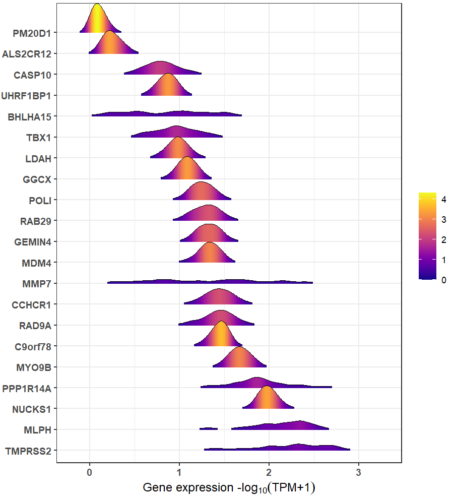

Trait gene MMP7 that with the highest PPH4.ABF=0.9978 & hypr_posterior=0.9993 encodes a member of the peptidase M10 family of matrix metalloproteinases, which is involved in the breakdown of extracellular matrix in normal physiological processes, such as embryonic development, reproduction, and tissue remodeling, as well as in disease processes, such as arthritis and metastasis. Prostate cancer can be promoted via MMP7-induced epithelial-to-mesenchymal transition by Interleukin-17. Resent literature has shown that serum MMP7 levels could guide metastatic therapy for prostate cancer.

Expression of MMP7 in multiple tissues can be plotted with xQTLvisual_geneExpTissues:

geneExpTissues <- xQTLvisual_geneExpTissues("MMP7", log10y = TRUE)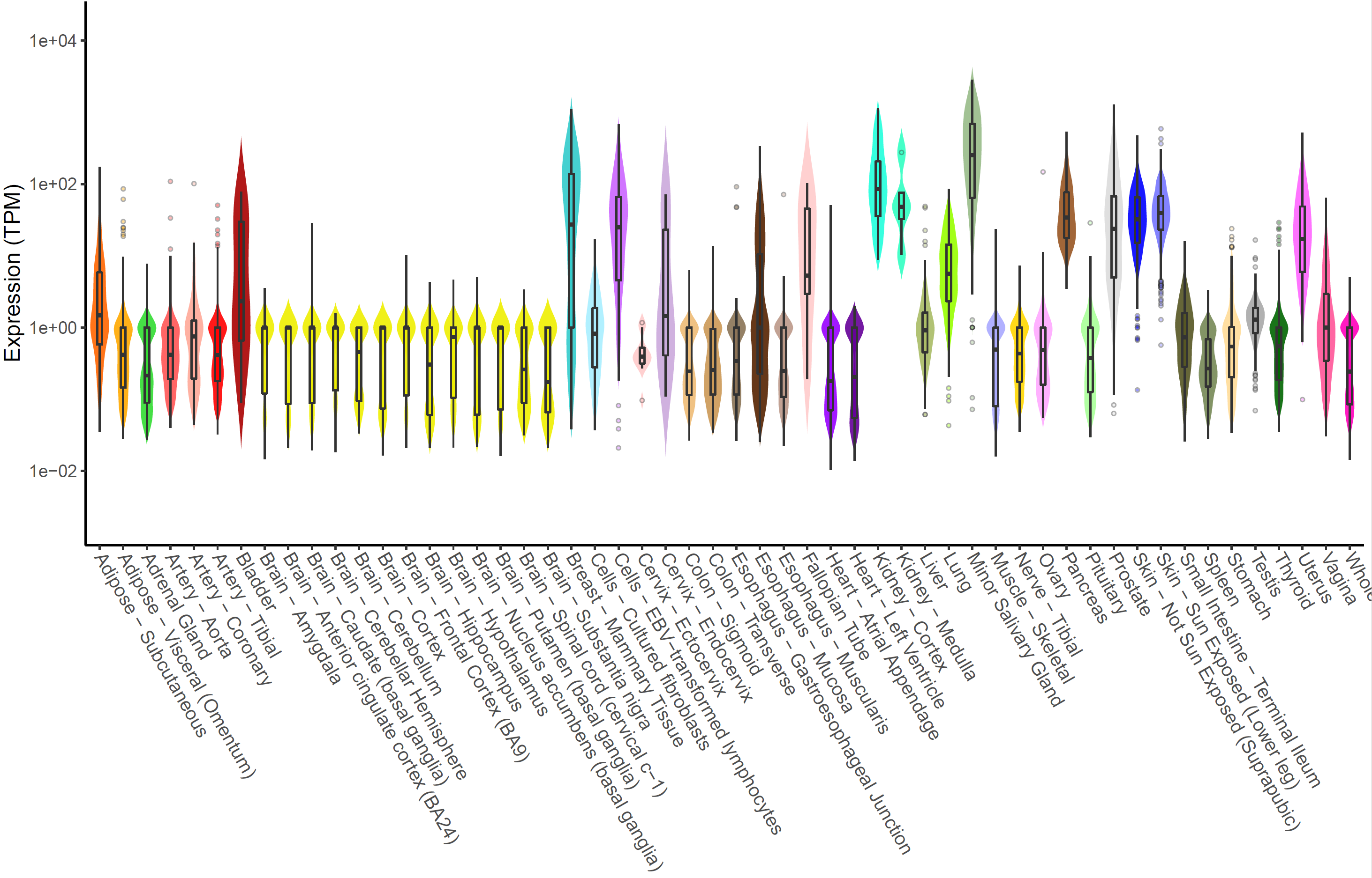

The number and significance of eQTLs in distinguished tissues are capable of showing a tissue-specific effect or a ubiquitous effect. The function xQTLvisual_eqtl can be used to indicate whether the gene is widely regulation in various tissues.

xQTLvisual_eqtl("MMP7")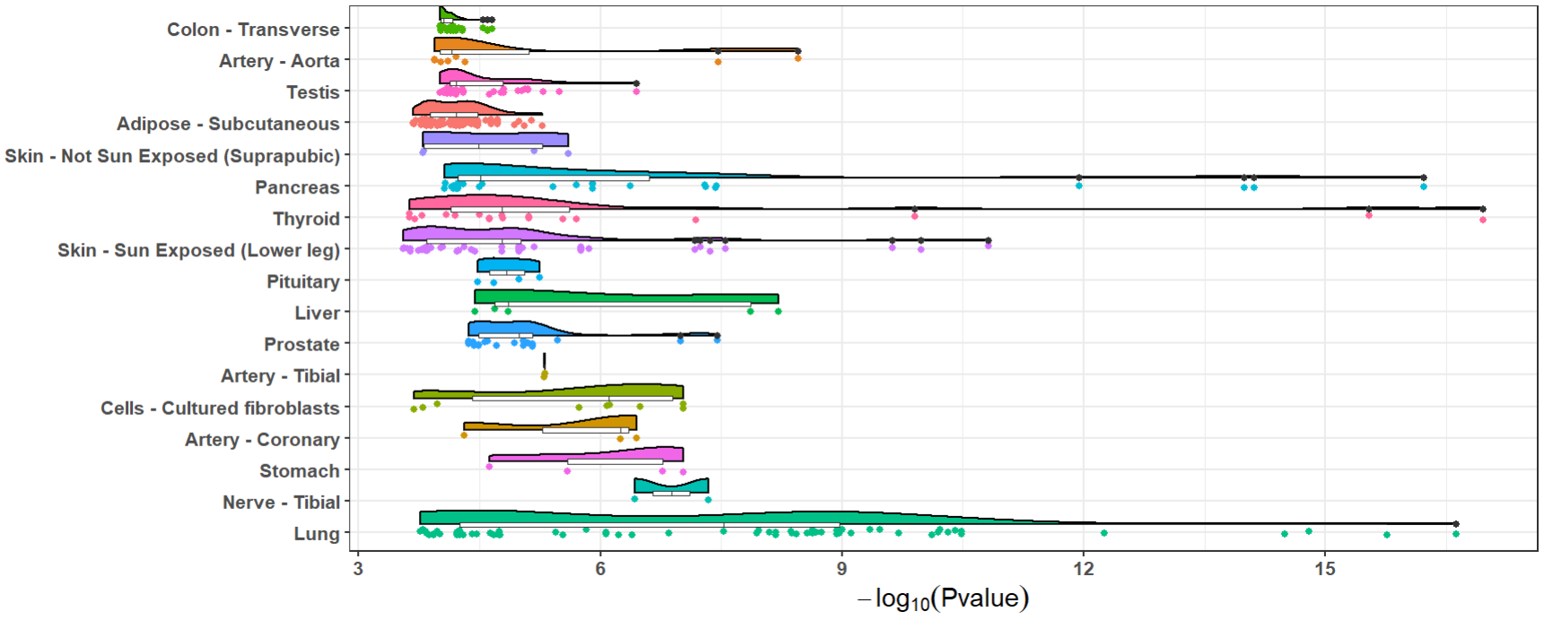

Besides, we provide functions xQTLvisual_locusCompare and xQTLvisual_locusZoom to visualize the colocalization between the GWAS and the eQTL dataset for a specified gene, we take the gene MMP7 as an example:

# Download all eQTL associations of gene  MMP7 in prostate:
eqtlAsso <- xQTLdownload_eqtlAllAsso(gene="MMP7",tissueLabel = tissueSiteDetail)
eqtlAsso <- data.table::as.data.table(eqtlAsso)
# Merge the variants of GWAS and eQTL dataset by rsid:
gwasEqtldata <- merge(gwasDF[,-c("AF")], eqtlAsso[,.(rsid=snpId, pValue)],
                      by=c("rsid"), suffixes = c(".gwas",".eqtl"))

Five retained fields are required:

gwasEqtldata

#>             rsid chrom  position pValue.gwas    beta     se pValue.eqtl
#>    1:  rs1004352    11 101777151   0.1901000 -0.0108 0.0083    0.175397
#>    2: rs10047467    11 101761011   0.4854000 -0.0096 0.0138    0.870120
#>    3: rs10047477    11 101696584   0.0791000  0.0147 0.0084    0.570213
#>    4: rs10047501    11 101696582   0.0755500 -0.0148 0.0083    0.570213
#>    5:  rs1006330    11 101626601   0.0564300  0.0169 0.0089    0.715533
#>   ---                                                                  
#> 7530:   rs996999    11 102667063   0.7268000 -0.0036 0.0102    0.309526
#> 7531:   rs998379    11 101587510   0.8520000 -0.0024 0.0126    0.156798
#> 7532:  rs9988826    11 101673906   0.7874000  0.0027 0.0101    0.117728
#> 7533:  rs9988861    11 101438758   0.0006782 -0.0306 0.0090    0.404080
#> 7534:  rs9988919    11 102876923   0.2217000  0.0331 0.0271    0.020295

Visualization of p-value distribution and comparison of the signals of GWAS and eQTL:

xQTLvisual_locusCompare(gwasEqtldata[,.(rsid, pValue.eqtl)], 
                        gwasEqtldata[,.(rsid, pValue.gwas)], legend_position = "bottomright")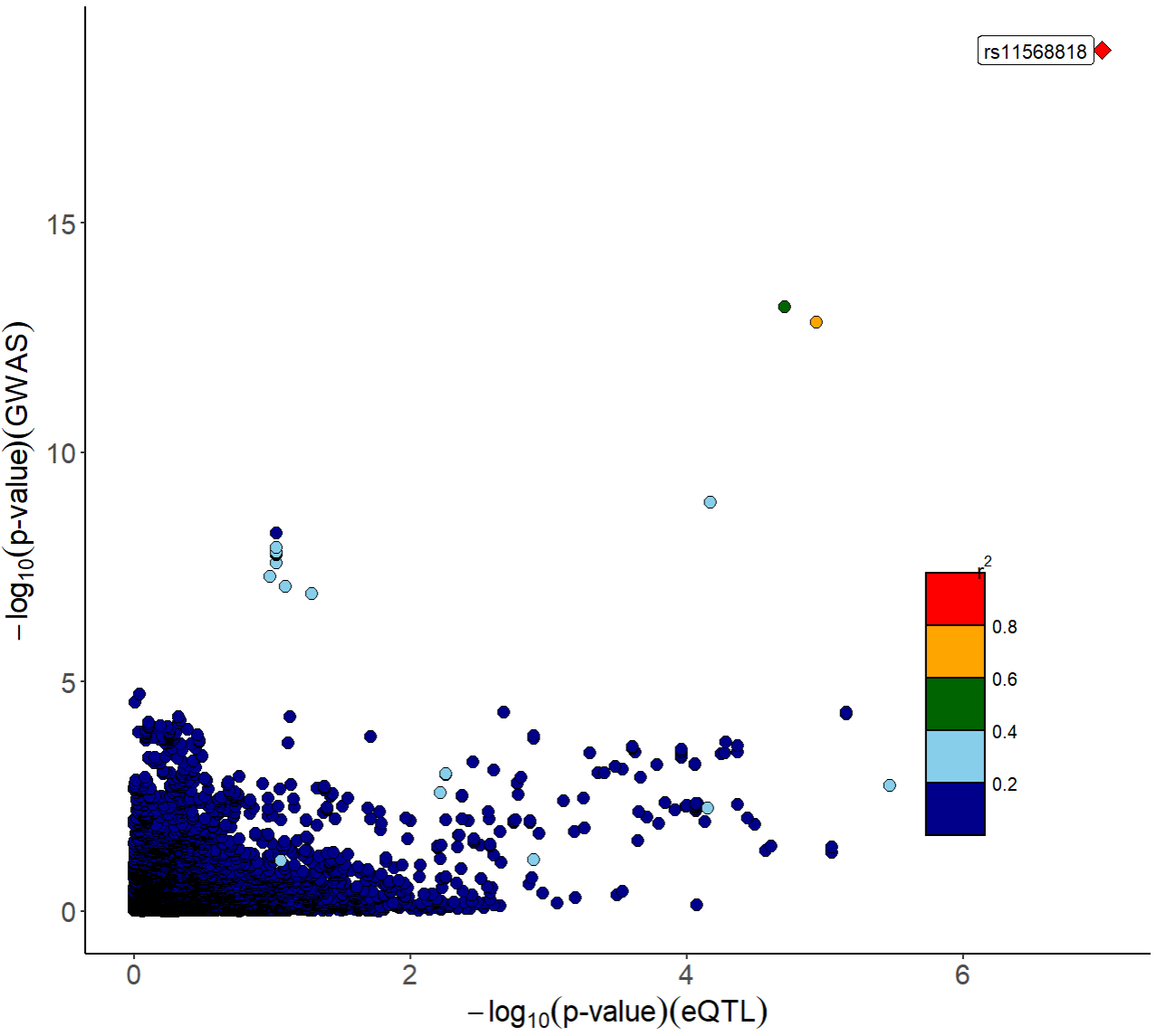

Locuszoom plot of GWAS signals:

xQTLvisual_locusZoom(gwasEqtldata[,.(rsid, chrom, position, pValue.gwas)], legend=FALSE)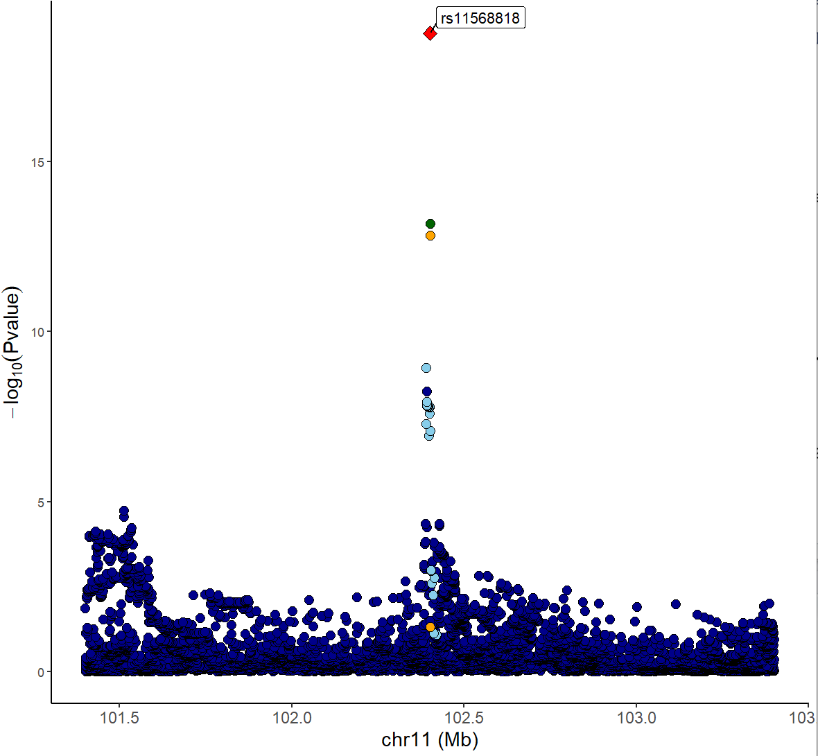

Locuszoom plot of eQTL signals:

xQTLvisual_locusZoom(gwasEqtldata[,.(rsid, chrom, position, pValue.eqtl)], legend=FALSE)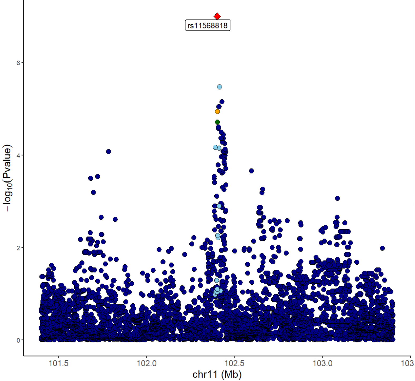

We can also combine locuscompare and locuszoom plot using function xQTLvisual_locusCombine:

xQTLvisual_locusCombine(gwasEqtldata[,c("rsid","chrom", "position", "pValue.gwas", "pValue.eqtl")])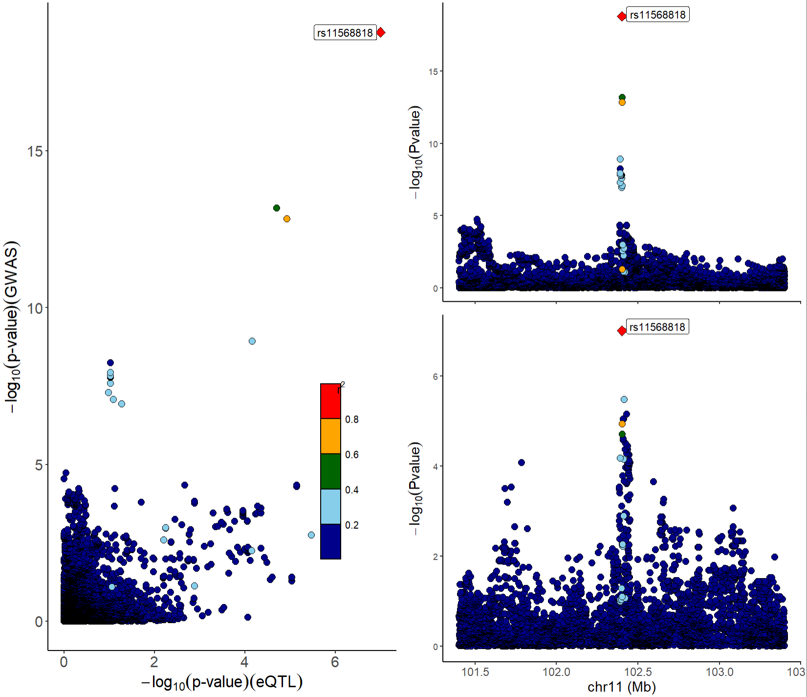

From the above figures, we can see that the SNP rs11568818 is potential causal variant, and we can use a violin plot to show the normalized effect size of it:

xQTLvisual_eqtlExp("rs11568818", "MMP7", tissueSiteDetail = tissueSiteDetail)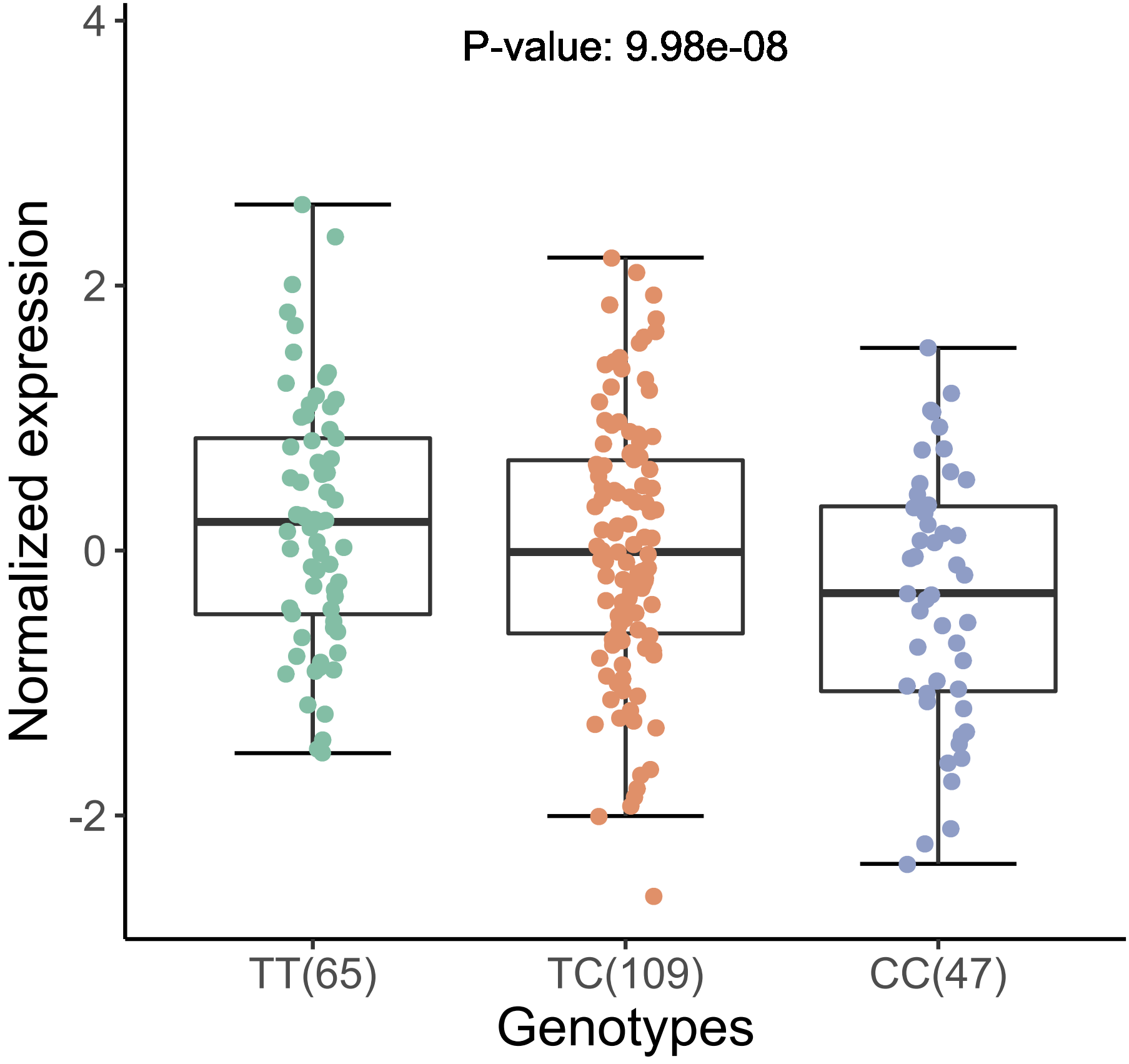

Extension: Integrative analysis with external packages or tools

To gain insight into the function of trait genes with higher PPH4, and explore the potential regulatory mechanism of the prostate cancer, we can conduct exploratory analysis, like co-expression analysis, and gene ontology enrichment analyses.

First we download expression profiles of the genes with higher value of PPH4 (>0.75) & hypr_posterior (>0.5) in prostate.

expMat <- xQTLdownload_exp(outGenes$gencodeId, tissueSiteDetail=tissueSiteDetail, toSummarizedExperiment =FALSE)

Pearson coefficient can be calculated with the expression matrix for each gene:

corDT <- cor(t(expMat[,-1:-7]))
colnames(corDT) <- outGenes$geneSymbol
rownames(corDT) <- outGenes$geneSymbol

R package corrplot is used to display this correlation matrix:

library(corrplot) 
corrplot(corDT, method="color",  
         type="upper",    
         order = "hclust",
         addCoef.col = "#ff0099", 
         number.cex = 0.7)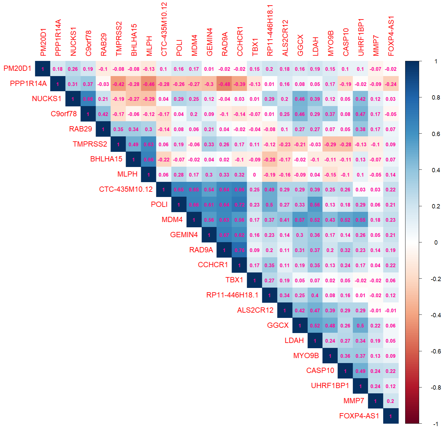

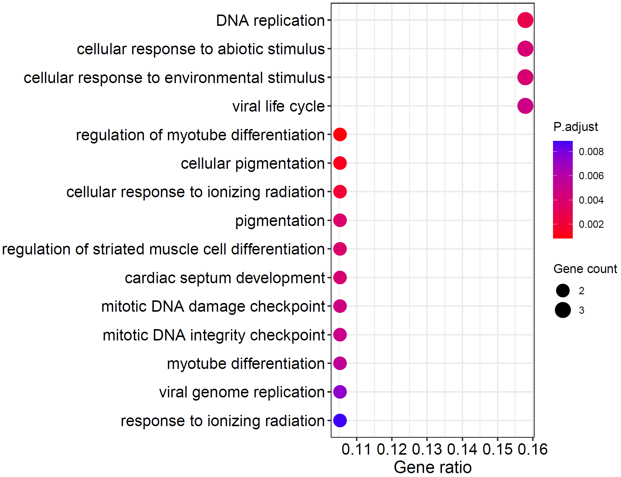
R package clusterProfiler is used for gene functional annotation: